How We Learned to Stop Guessing and Love Low P-Values
February 8, 2021
“I don’t think it’s quite fair to condemn the whole program because of a single slip up, sir.” Famous last words from Kubrick’s 1964 classic Dr. Strangelove, as a forlorn general realizes his negligence is about to lead to nuclear apocalypse. This may feel relatable to any engineer who has immediately regretted pushing the big red “release” button only to later find themselves putting out fires late into the night. Sometimes the answer is simply “write more tests!” or “write better tests!”, but for matters of performance, it’s not so simple.
Users of YugabyteDB are consistently delighted by our performance and appreciate further improvements we consistently make on this front. Ensuring we maintain our high performance bar as we continue to add new features is of paramount importance to us. But doing so in a rigorous manner is not as straightforward as you might hope.
So what’s the problem? Measure it!
How often should we measure performance? We could do so only when we make changes in the critical path, but what if seemingly unrelated changes affect translation unit boundaries, and your compiler optimizations are affected? What if you are consistently making changes to the critical path because you’re constantly trying to deliver better performance for your users? Getting into the business of predicting which changes will affect performance can be dangerous. In most cases, you should be regularly testing for performance regressions. With regular commits from over 100 contributors, we’ve opted to measure this nightly, and for changes we expect to directly impact performance, we additionally measure and evaluate before committing.
How should we measure performance? Many of our users run YugabyteDB on virtual machines, so that would be the most realistic environment, but VMs are shared and access to resources can be variable. In addition, the network is inconsistent. In a storage system like YugabyteDB, even things like background compactions can impact performance in an unpredictable or seemingly inconsistent way.
Once we measure, how do we interpret? Direct comparisons of measurements between two runs can be incredibly noisy. Worse still, if a change is blocked on such an evaluation, we can surely expect that the engineer who is responsible for evaluating the impact of their own change will be as biased as our process allows them to be.
Beer to the rescue!
Well, kind of. In 1908, publishing under the pseudonym “Student” while working at a Guinness factory, William Gosset shared the statistical insights he used to compute robust confidence intervals around various yield metrics of Guinness stout (say, ABV) using small sample sizes. But we’re not interested in making beer. We’re interested in drinking it! What I mean to say is, we’re interested in database performance!
Let’s say you’ve just created a new build, which includes your changes to improve latency to one of your microservices, on top of the master branch. You’ve generated a dataset of statistically independent latency measurements. The data seems like an improvement, but you’ve learned to stop guessing (and soon, you will learn to love low p-values). As it turns out, you can use the same principles used by Gosset to make quality beer to quickly determine if the latency data you generated is in fact a statistically significant improvement. Ready your beers — we’re about to prove that you just reduced latency!
The framework that follows is broadly termed “statistical hypothesis testing,” of which Student’s t-test is an example. Let’s do some math — assuming A = a_1, … a_n are independent, identically distributed random variables, in this case tracking latency measurements, let S = stddev(A). Then \frac{avg(A) - \mu}{\frac{S}{\sqrt{n}}} is normally distributed with mean 0 and variance 1.
This is a very basic re-statement of the central limit theorem (CLT), which assumes large samples of statistically independent data (note: we will address these assumptions below). Now, supposing A is a sample of latencies, the CLT makes computing a confidence interval of latencies for our build easy. But for our scenario, we want to answer a slightly different question — “given two samples of latencies, one generated from a master build, and another generated from your build, how confident can we be that your build is truly an improvement?”
Consider two samples of latencies which we assume to be drawn from independent normal distributions. One is your baseline sample, and another the sample generated from your new build.
A = a_1, a_2, ... a_n \sim \mathcal{N}(\mu_A,\,\sigma_A^{2})B = b_1, b_2, ... b_m \sim \mathcal{N}(\mu_B,\,\sigma_B^{2})Let D = \mu_A - \mu_B (difference of true, unobserved means), D^\star = avg(A) - avg(B) (difference of observed means), S_A, S_B are the observed standard deviations of A and B, respectively. Then, applying the CLT to A - B, we can say the following:
\frac{D – D^\star}{\sqrt{\frac{S_A^2}{n} + \frac{S_B^2}{m}}} \sim \mathcal{N}(0, 1)A-ha! As we’re about to see, this fact is very useful to us. We’ve constructed a random variable with the quantity of interest D = \mu_A – \mu_B which follows a known distribution. Namely:
\text{Let } Z = \frac{|D – D^\star|}{\sqrt{\frac{S_A^2}{n} + \frac{S_B^2}{m}}} \text{, then, } \mathsf{P}(Z \geq x) = \mathsf{P}(|\mathcal{N}(0, 1)| \geq x)Our baseline assumption, or so-called null hypothesis, is that our change did not meaningfully improve or regress performance — in other words, D = \mu_A - \mu_B = 0. So, we then ask the question, “assuming these builds perform identically, how likely are we to observe the data we have generated?” In mathematical terms, this question can be expressed as follows, and the answer to this question is called our p-value:
Let Z’ = \frac{|avg(A) - avg(B)|}{\sqrt{\frac{S_A^2}{n} + \frac{S_B^2}{m}}}
Then p = P(|N(0,1)| >= Z’)
If the answer to this question, our p-value, is very low, then we can confidently reject our null hypothesis. In other words, the probability of these two builds performing identically in the long run is low. In other words, a low p-value, and a high decrease in observed average latency, means we can be pretty confident your change is truly an improvement!
Putting it to use
In practice, you need to be careful that your latency data respect all the assumptions our math is making. For example, ensuring data in your sample are statistically independent can be hard. A naive approach of measuring consecutive latencies from a single workload run can be problematic — in real-world systems, sources of noise are often temporally correlated. A full treatment of the means in which one would generate independent observations is enough to fill another blog post.
Having large enough samples to directly apply the CLT is also hard. This is where our Guinness hero comes in. Student’s t-test was specifically formulated to give accurate statistical confidence measurements when dealing with small samples. In practice, if your data generated are in fact generated independently, your sample sizes will likely be small. Unfortunately the math for Student’s t-test is a bit messier, so we’ve outlined the more general and easier-to-follow framework above, but the approach is fundamentally the same. At any rate, you should rely on an existing library (see e.g. scipy, benchstat, Apache commons) where possible, rather than rolling your own.
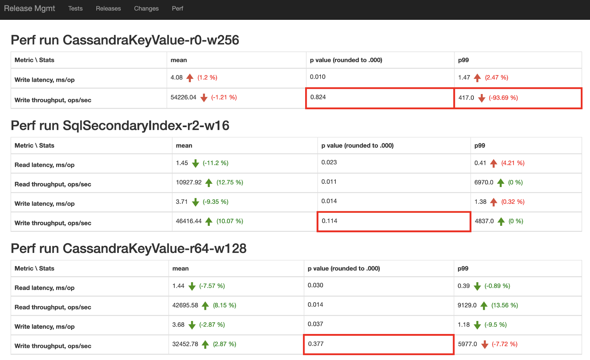
At Yugabyte, we have nightly runs which store samples of various performance metrics (read latency, write throughput, etc.) for various workloads, so that any future nightly run can be compared to any past run easily. We display such comparisons in a UI that looks like this, with regressions and high p-values highlighted:
Armed with the power of statistics, you too can avoid human bias, stop guessing, and learn to love low p-values!


